-
Notifications
You must be signed in to change notification settings - Fork 25
/
Clustering.md
570 lines (486 loc) · 20.7 KB
/
Clustering.md
1
2
3
4
5
6
7
8
9
10
11
12
13
14
15
16
17
18
19
20
21
22
23
24
25
26
27
28
29
30
31
32
33
34
35
36
37
38
39
40
41
42
43
44
45
46
47
48
49
50
51
52
53
54
55
56
57
58
59
60
61
62
63
64
65
66
67
68
69
70
71
72
73
74
75
76
77
78
79
80
81
82
83
84
85
86
87
88
89
90
91
92
93
94
95
96
97
98
99
100
101
102
103
104
105
106
107
108
109
110
111
112
113
114
115
116
117
118
119
120
121
122
123
124
125
126
127
128
129
130
131
132
133
134
135
136
137
138
139
140
141
142
143
144
145
146
147
148
149
150
151
152
153
154
155
156
157
158
159
160
161
162
163
164
165
166
167
168
169
170
171
172
173
174
175
176
177
178
179
180
181
182
183
184
185
186
187
188
189
190
191
192
193
194
195
196
197
198
199
200
201
202
203
204
205
206
207
208
209
210
211
212
213
214
215
216
217
218
219
220
221
222
223
224
225
226
227
228
229
230
231
232
233
234
235
236
237
238
239
240
241
242
243
244
245
246
247
248
249
250
251
252
253
254
255
256
257
258
259
260
261
262
263
264
265
266
267
268
269
270
271
272
273
274
275
276
277
278
279
280
281
282
283
284
285
286
287
288
289
290
291
292
293
294
295
296
297
298
299
300
301
302
303
304
305
306
307
308
309
310
311
312
313
314
315
316
317
318
319
320
321
322
323
324
325
326
327
328
329
330
331
332
333
334
335
336
337
338
339
340
341
342
343
344
345
346
347
348
349
350
351
352
353
354
355
356
357
358
359
360
361
362
363
364
365
366
367
368
369
370
371
372
373
374
375
376
377
378
379
380
381
382
383
384
385
386
387
388
389
390
391
392
393
394
395
396
397
398
399
400
401
402
403
404
405
406
407
408
409
410
411
412
413
414
415
416
417
418
419
420
421
422
423
424
425
426
427
428
429
430
431
432
433
434
435
436
437
438
439
440
441
442
443
444
445
446
447
448
449
450
451
452
453
454
455
456
457
458
459
460
461
462
463
464
465
466
467
468
469
470
471
472
473
474
475
476
477
478
479
480
481
482
483
484
485
486
487
488
489
490
491
492
493
494
495
496
497
498
499
500
501
502
503
504
505
506
507
508
509
510
511
512
513
514
515
516
517
518
519
520
521
522
523
524
525
526
527
528
529
530
531
532
533
534
535
536
537
538
539
540
541
542
543
544
545
546
547
548
549
550
551
552
553
554
555
556
557
558
559
560
561
562
563
564
565
566
567
568
569
570
# Clustering
Cluster analysis itself is not one specific algorithm, but the general task to be solved. It can be achieved by various algorithms that differ significantly in their understanding of what constitutes a cluster and how to efficiently find them. Popular notions of clusters include groups with small distances between cluster members, dense areas of the data space, intervals or particular statistical distributions. Clustering can therefore be formulated as a multi-objective optimization problem. The appropriate clustering algorithm and parameter settings (including parameters such as the distance function to use, a density threshold or the number of expected clusters) depend on the individual data set and intended use of the results. Cluster analysis as such is not an automatic task, but an iterative process of knowledge discovery or interactive multi-objective optimization that involves trial and failure. It is often necessary to modify data preprocessing and model parameters until the result achieves the desired properties.
## Table of Contents
- [1. Data Preparation](#data-preparation)
- [2. Model Selection](#model-selection)
- [3. Data Results](#data-results)
## Data Preparation
After installing it, the first step is to run the Geochemistry Pi framework in your terminal application.
In this section, we take the built-in dataset as an example by running:
geochemistrypi data-mining
Alternatively, it is perfectly fine if you would like to use your own dataset like:
geochemistrypi data-mining --data your_own_data_set.xlsx
You can choose the appropriate option based on the program’s prompts and press the Enter key to select the default option (inside the parentheses).
Welcome to Geochemistry π!
Initializing...
No Training Data File Provided!
Built-in Data Loading.
No Application Data File Provided!
Built-in Application Data Loading.
Downloading Basemap...
...
Successfully downloading!
Download happens only once!
(Press Enter key to move forward.)
✨ Press Ctrl + C to exit our software at any time.
✨ Input Template [Option1/Option2] (Default Value): Input Value
✨ Use Previous Experiment [y/n] (n): >Enter
✨ New Experiment (GeoPi - Rock Classification): GeoPi - Rock Clustering
✨ Run Name (XGBoost Algorithm - Test 1):>Enter
(Press Enter key to move forward.)
After pressing the Enter key, the program propts the following options to let you **choose the Built-in Training Data**:
-*-*- Built-in Training Data Option-*-*-
1 - Data For Regression
2 - Data For Classification
3 - Data For Clustering
4 - Data For Dimensional Reduction
(User) ➜ @Number:3
Here, we choose *3 - Data For Clustering* and press the Enter key to move forward.
Now, you should see the output below on your screen:
Successfully loading the built-in training data set 'Data_Clustering.xlsx'.
--------------------
Index - Column Name
1 - CITATION
2 - SAMPLE NAME
3 - Label
4 - Notes
5 - LATITUDE
...
41 - YB(PPM)
42 - LU(PPM)
43 - HF(PPM)
44 - TA(PPM)
45 - PB(PPM)
46 - TH(PPM)
47 - U(PPM)
--------------------
(Press Enter key to move forward.)
We hit Enter key to keep moving.
Then, we choose *2 - Data For Clustering* as our **Built-in Application Data**:
-*-*- Built-in Application Data Option-*-*-
1 - Data For Regression
2 - Data For Classification
3 - Data For Clustering
4 - Data For Dimensional Reduction
(User) ➜ @Number: 3
After this, the program will display a list for Column Name:
Successfully loading the built-in inference data set
'InferenceData_Clustering.xlsx'.
--------------------
Index - Column Name
1 - CITATION
2 - SAMPLE NAME
3 - Label
4 - Notes
5 - LATITUDE
6 - LONGITUDE
7 - Unnamed: 6
8 - SIO2(WT%)
9 - TIO2(WT%)
10 - AL2O3(WT%)
11 - CR2O3(WT%)
12 - FEOT(WT%)
13 - CAO(WT%)
14 - MGO(WT%)
15 - MNO(WT%)
16 - NA2O(WT%)
17 - Unnamed: 16
18 - SC(PPM)
19 - TI(PPM)
20 - V(PPM)
21 - CR(PPM)
22 - NI(PPM)
23 - RB(PPM)
24 - SR(PPM)
25 - Y(PPM)
26 - ZR(PPM)
27 - NB(PPM)
28 - BA(PPM)
29 - LA(PPM)
30 - CE(PPM)
31 - PR(PPM)
32 - ND(PPM)
33 - SM(PPM)
34 - EU(PPM)
35 - GD(PPM)
36 - TB(PPM)
37 - DY(PPM)
38 - HO(PPM)
39 - ER(PPM)
40 - TM(PPM)
41 - YB(PPM)
42 - LU(PPM)
43 - HF(PPM)
44 - TA(PPM)
45 - PB(PPM)
46 - TH(PPM)
47 - U(PPM)
--------------------
(Press Enter key to move forward.)
After pressing the Enter key, you can choose whether you need a world map projection for a specific element option:
-*-*- World Map Projection -*-*-
World Map Projection for A Specific Element Option:
1 - Yes
2 - No
(Plot) ➜ @Number:
More information of the map projection can be found in the section of World Map Projection. In this tutorial, we skip it by typing 2 and pressing the Enter key.
### Data Selection
And, we include column 8, 9, 10, 11, 12, 13 (i.e. [8, 13]) in our example.
-*-*- Data Selection -*-*-
--------------------
Index - Column Name
1 - CITATION
2 - SAMPLE NAME
3 - Label
4 - Notes
5 - LATITUDE
6 - LONGITUDE
7 - Unnamed: 6
8 - SIO2(WT%)
9 - TIO2(WT%)
10 - AL2O3(WT%)
11 - CR2O3(WT%)
12 - FEOT(WT%)
13 - CAO(WT%)
...
47 - U(PPM)
--------------------
Select the data range you want to process.
Input format:
Format 1: "[**, **]; **; [**, **]", such as "[1, 3]; 7; [10, 13]" --> you want to deal with the columns 1, 2, 3, 7, 10, 11, 12, 13
Format 2: "xx", such as "7" --> you want to deal with the columns 7
@input: [8,13]
Have a double-check on your selection and press Enter to move forward:
--------------------
Index - Column Name
8 - SIO2(WT%)
9 - TIO2(WT%)
10 - AL2O3(WT%)
11 - CR2O3(WT%)
12 - FEOT(WT%)
13 - CAO(WT%)
--------------------
(Press Enter key to move forward.)
The Selected Data Set:
SIO2(WT%) TIO2(WT%) AL2O3(WT%) CR2O3(WT%) FEOT(WT%) CAO(WT%)
0 53.640000 0.400000 0.140000 0.695000 11.130000 20.240000
1 52.740000 0.386000 0.060000 0.695000 12.140000 20.480000
2 51.710000 0.730000 2.930000 0.380000 6.850000 22.420000
3 50.870000 0.780000 2.870000 0.640000 7.530000 22.450000
4 50.920000 0.710000 2.900000 0.300000 6.930000 22.620000
... ... ... ... ... ... ...
2006 52.628866 0.409385 5.612482 0.606707 2.202400 21.172240
2007 52.535656 0.422012 5.384972 1.278862 2.093113 21.150105
2008 52.163411 0.665545 4.965511 0.667931 2.202465 21.600643
2009 44.940000 3.930000 8.110000 0.280000 6.910000 22.520000
2010 46.750000 3.360000 6.640000 0.000000 7.550000 22.540000
[2011 rows x 6 columns]
(Press Enter key to move forward.)
Now, you should see
-*-*- Basic Statistical Information -*-*-
<class 'pandas.core.frame.DataFrame'>
RangeIndex: 2011 entries, 0 to 2010
Data columns (total 6 columns):
# Column Non-Null Count Dtype
--- ------ -------------- -----
0 SIO2(WT%) 2011 non-null float64
1 TIO2(WT%) 2011 non-null float64
2 AL2O3(WT%) 2011 non-null float64
3 CR2O3(WT%) 2011 non-null float64
4 FEOT(WT%) 2011 non-null float64
5 CAO(WT%) 2011 non-null float64
dtypes: float64(6)
memory usage: 94.4 KB
None
Some basic statistic information of the designated data set:
SIO2(WT%) TIO2(WT%) AL2O3(WT%) CR2O3(WT%) FEOT(WT%) CAO(WT%)
count 2011.000000 2011.000000 2011.000000 2011.000000 2011.000000 2011.000000
mean 52.110416 0.411454 4.627858 0.756601 3.215889 21.442025
std 2.112777 0.437279 2.268114 0.581543 1.496576 2.325046
min 0.218000 0.000000 0.010000 0.000000 1.281000 0.097000
25% 51.350271 0.166500 3.531000 0.490500 2.535429 20.532909
50% 52.200000 0.320000 4.923000 0.695000 2.920000 21.600000
75% 52.980000 0.512043 5.921734 0.912950 3.334500 22.421935
max 56.301066 6.970000 48.223000 15.421000 18.270000 26.090000
Successfully calculate the pair-wise correlation coefficient among the selected
columns.
...
Successfully...
Successfully...
...
Successfully store 'Data Selected' in 'Data Selected.xlsx' in C:\Users\YSQ\geopi_output\GeoPi - Rock Clustering\XGBoost Algorithm - Test 1\artifacts\data.
(Press Enter key to move forward.)
You should now see a lot of output on your screen, but don’t panic.
This output just documents the successful execution of tasks such as calculating correlations, drawing distribution plots, and saving generated charts and data files.
Now, let’s press the Enter key to proceed.
-*-*- Missing Value Check -*-*-
Check which column has null values:
--------------------
SIO2(WT%) False
TIO2(WT%) False
AL2O3(WT%) False
CR2O3(WT%) False
FEOT(WT%) False
CAO(WT%) False
dtype: bool
--------------------
The ratio of the null values in each column:
--------------------
SIO2(WT%) 0.0
TIO2(WT%) 0.0
AL2O3(WT%) 0.0
CR2O3(WT%) 0.0
FEOT(WT%) 0.0
CAO(WT%) 0.0
dtype: float64
--------------------
Note: The provided data set is complete without missing values, we'll just pass this
step!
Successfully store 'Data Selected Dropped-Imputed' in 'Data Selected
Dropped-Imputed.xlsx' in C:\Users\YSQ\geopi_output\GeoPi - Rock Clustering\XGBoost
Algorithm - Test 1\artifacts\data.
(Press Enter key to move forward.)
According to the note, the dataset is complete without missing values, we'll just pass this step!
### Feature Engineering
The next step is to select your feature engineering options, for simplicity, we omit the specific operations here. For detailed instructions, please see the document "Decomposition".
-*-*- Feature Engineering -*-*-
The Selected Data Set:
--------------------
Index - Column Name
1 - SIO2(WT%)
2 - TIO2(WT%)
3 - AL2O3(WT%)
4 - CR2O3(WT%)
5 - FEOT(WT%)
6 - CAO(WT%)
--------------------
Feature Engineering Option:
1 - Yes
2 - No
(Data) ➜ @Number:2
> Enter
Successfully store 'Data Selected Dropped-Imputed Feature-Engineering' in 'Data
Selected Dropped-Imputed Feature-Engineering.xlsx' in
C:\Users\YSQ\geopi_output\GeoPi - Rock Clustering\XGBoost Algorithm - Test
1\artifacts\data.
(Press Enter key to move forward.)
## Model Selection
This version of geochemistrypi provide 2 clustering models: Kmeans and DBSCN. Both of them are popular algorithms used for clustering problems. Here we use Kmeans as an example.
-*-*- Model Selection -*-*-:
1 - KMeans
2 - DBSCAN
3 - Agglomerative
4 - All models above to be trained
Which model do you want to apply?(Enter the Corresponding Number)
(Model) ➜ @Number: 1
### Hyper-Parameters Specification
Before starting the training process, you have to specify the number of clusters for our kmeans model:
-*-*- Hyper-parameters Specification -*-*-
N Clusters Number: The number of clusters to form as well as the number of centroids to generate.
Please specify the number of clusters for KMeans. A good starting range could be between 2 and 10, such as 4.
(Model) ➜ N Clusters: 5
Then,choose the method for initialization of centroids. Here, we choose method 1.
Init: Method for initialization of centroids. The centroids represent the center points of the clusters in the dataset.
Please specify the method for initialization of centroids. It is generally recommended to leave it as 'k-means++'.
1 - k-means++
2 - random
(Model) ➜ @Number:1
The max_iter parameter in the K-means algorithm represents the maximum number of iterations. This parameter specifies the number of attempts the algorithm will make to cluster the data points before stopping, even if the clustering has not yet converged. Initially, a relatively small value can be chosen, and then gradually increased until the desired convergence criteria are met.
Max Iter: Maximum number of iterations of the k-means algorithm for a single run.
Please specify the maximum number of iterations of the k-means algorithm for a single run. A good starting range could
be between 100 and 500, such as 300.
(Model) ➜ Max Iter:300
Setting the tolerance value in clustering algorithms is to specify the precision or error range required for the algorithm to converge.
Tolerance: Relative tolerance with regards to inertia to declare convergence.
Please specify the relative tolerance with regards to inertia to declare convergence. A good starting range could be
between 0.0001 and 0.001, such as 0.0005.
(Model) ➜ Tolerance:0.0005
Then, we need to choose algorithm. Here, we use auto.
Algorithm: The algorithm to use for the computation.
Please specify the algorithm to use for the computation. It is generally recommended to leave it as 'auto'.
Auto: selects 'elkan' for dense data and 'full' for sparse data. 'elkan' is generally faster on data with lower
dimensionality, while 'full' is faster on data with higher dimensionality
1 - auto
2 - full
3 - elkan
(Model) ➜ @Number:1
(Press Enter key to move forward.)
> Enter
Then you can start to run the kmeans model with your dataset.
## Data Results
The clustering reuslt will bu printed and saved to the output/data directory.
```
*-**-* KMeans is running ... *-**-*
Expected Functionality:
+ Cluster Centers
+ Cluster Labels
+ Model Persistence
+ KMeans Score
-----* Clustering Centers *-----
[[5.41388401e+01 2.15829364e-01 1.29914717e+00 4.67482921e-01
3.19637435e+00 2.35938062e+01]
[5.22315058e+01 3.33761788e-01 4.56573367e+00 8.00137780e-01
3.03767947e+00 2.14858778e+01]
[4.47251667e+01 5.05000000e-02 1.58216667e+00 9.81666667e-02
9.22933333e+00 4.75750000e-01]
[5.08836094e+01 6.82282120e-01 6.77641282e+00 8.42755279e-01
3.40927321e+00 2.05098654e+01]
[2.18000000e-01 1.63000000e-01 4.82230000e+01 1.54210000e+01
1.54690000e+01 1.09000000e-01]]
-----* Clustering Labels *-----
clustering result
0 0
1 0
2 1
3 1
4 1
... ...
2006 1
2007 1
2008 1
2009 3
2010 3
[2011 rows x 1 columns]
Successfully store 'KMeans Result' in 'KMeans Result.xlsx' in C:\Users\YSQ\geopi_output\n\test2\artifacts\data.
Successfully store 'Hyper Parameters - KMeans' in 'Hyper Parameters - KMeans.txt' in
C:\Users\YSQ\geopi_output\n\test2\parameters.
-----* Model Score *-----
silhouette_score: 0.30630378777495465
calinski_harabasz_score: 924.9161281178593
Successfully store 'Model Score - KMeans' in 'Model Score - KMeans.txt' in C:\Users\YSQ\geopi_output\n\test2\metrics.
```
### 2 dimensions graphs of data
choose two demensions of data to draw the plot.
```
-----* 2 Dimensions Data Selection *-----
The software is going to draw related 2d graphs.
Currently, the data dimension is beyond 2 dimensions.
Please choose 2 dimensions of the data below.
1 - SIO2(WT%)
2 - TIO2(WT%)
3 - AL2O3(WT%)
4 - CR2O3(WT%)
5 - FEOT(WT%)
6 - CAO(WT%)
Choose dimension - 1 data:
(Plot) ➜ @Number:1
1 - SIO2(WT%)
2 - TIO2(WT%)
3 - AL2O3(WT%)
4 - CR2O3(WT%)
5 - FEOT(WT%)
6 - CAO(WT%)
Choose dimension - 2 data:
(Plot) ➜ @Number:2
The Selected Data Dimension:
--------------------
Index - Column Name
1 - SIO2(WT%)
2 - TIO2(WT%)
--------------------
-----* Clustering Centers *-----
[[5.41388401e+01 2.15829364e-01 1.29914717e+00 4.67482921e-01
3.19637435e+00 2.35938062e+01]
[5.22315058e+01 3.33761788e-01 4.56573367e+00 8.00137780e-01
3.03767947e+00 2.14858778e+01]
[4.47251667e+01 5.05000000e-02 1.58216667e+00 9.81666667e-02
9.22933333e+00 4.75750000e-01]
[5.08836094e+01 6.82282120e-01 6.77641282e+00 8.42755279e-01
3.40927321e+00 2.05098654e+01]
[2.18000000e-01 1.63000000e-01 4.82230000e+01 1.54210000e+01
1.54690000e+01 1.09000000e-01]]
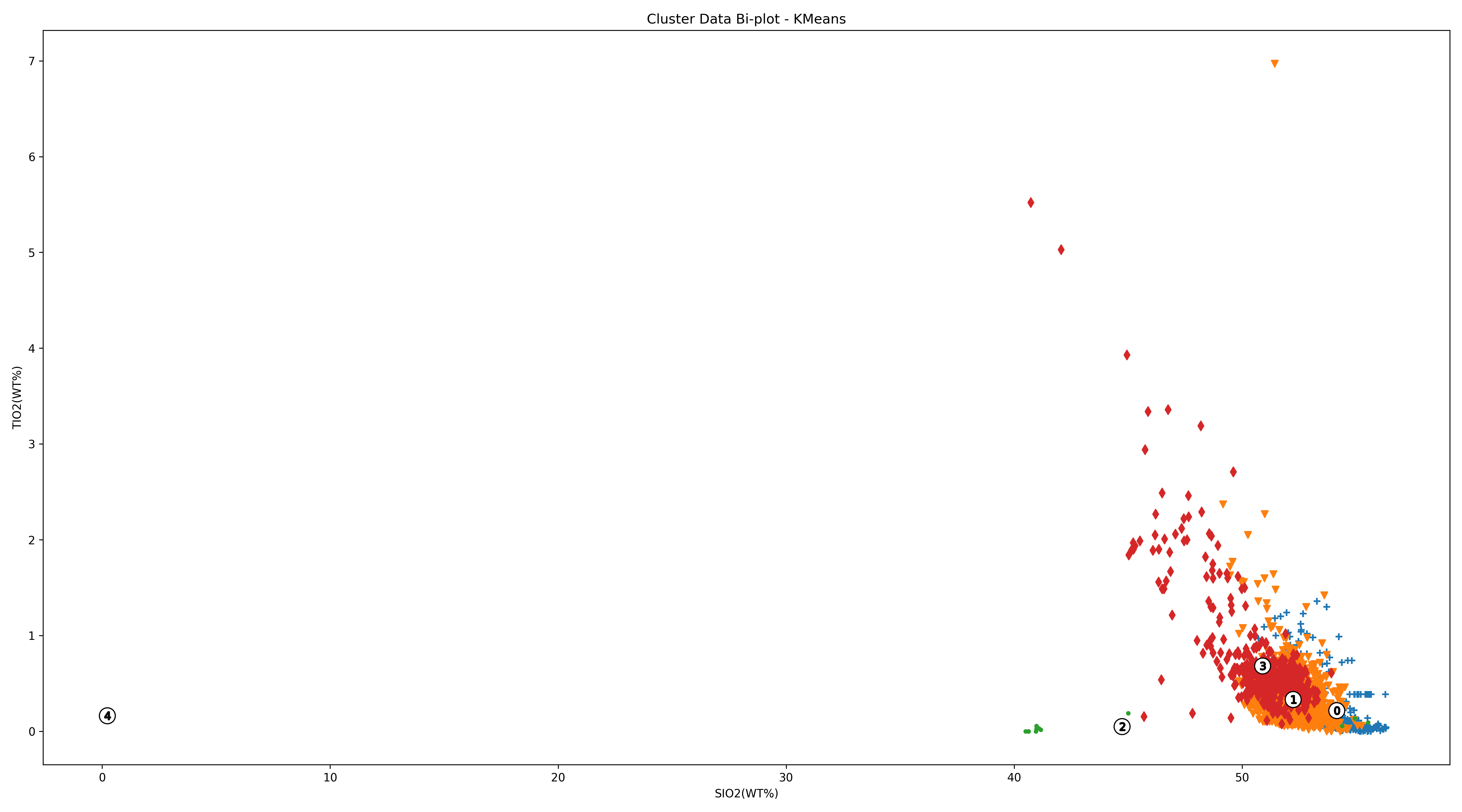
-----* Cluster Two-Dimensional Diagram *-----
Save figure 'Cluster Two-Dimensional Diagram - KMeans' in
C:\Users\YSQ\geopi_output\n\test2\artifacts\image\model_output.
Successfully store 'Cluster Two-Dimensional Diagram - KMeans' in 'Cluster Two-Dimensional Diagram - KMeans.xlsx' in
C:\Users\YSQ\geopi_output\n\test2\artifacts\image\model_output.
```
### 3 dimensions graphs of data
choose three columns of data to draw the plot.
```
-----* 3 Dimensions Data Selection *-----
The software is going to draw related 3d graphs.
Currently, the data dimension is beyond 3 dimensions.
Please choose 3 dimensions of the data below.
1 - SIO2(WT%)
2 - TIO2(WT%)
3 - AL2O3(WT%)
4 - CR2O3(WT%)
5 - FEOT(WT%)
6 - CAO(WT%)
Choose dimension - 1 data:
(Plot) ➜ @Number: 2
1 - SIO2(WT%)
2 - TIO2(WT%)
3 - AL2O3(WT%)
4 - CR2O3(WT%)
5 - FEOT(WT%)
6 - CAO(WT%)
Choose dimension - 2 data:
(Plot) ➜ @Number: 3
1 - SIO2(WT%)
2 - TIO2(WT%)
3 - AL2O3(WT%)
4 - CR2O3(WT%)
5 - FEOT(WT%)
6 - CAO(WT%)
Choose dimension - 3 data:
(Plot) ➜ @Number: 4
The Selected Data Dimension:
--------------------
Index - Column Name
1 - TIO2(WT%)
2 - AL2O3(WT%)
3 - CR2O3(WT%)
--------------------
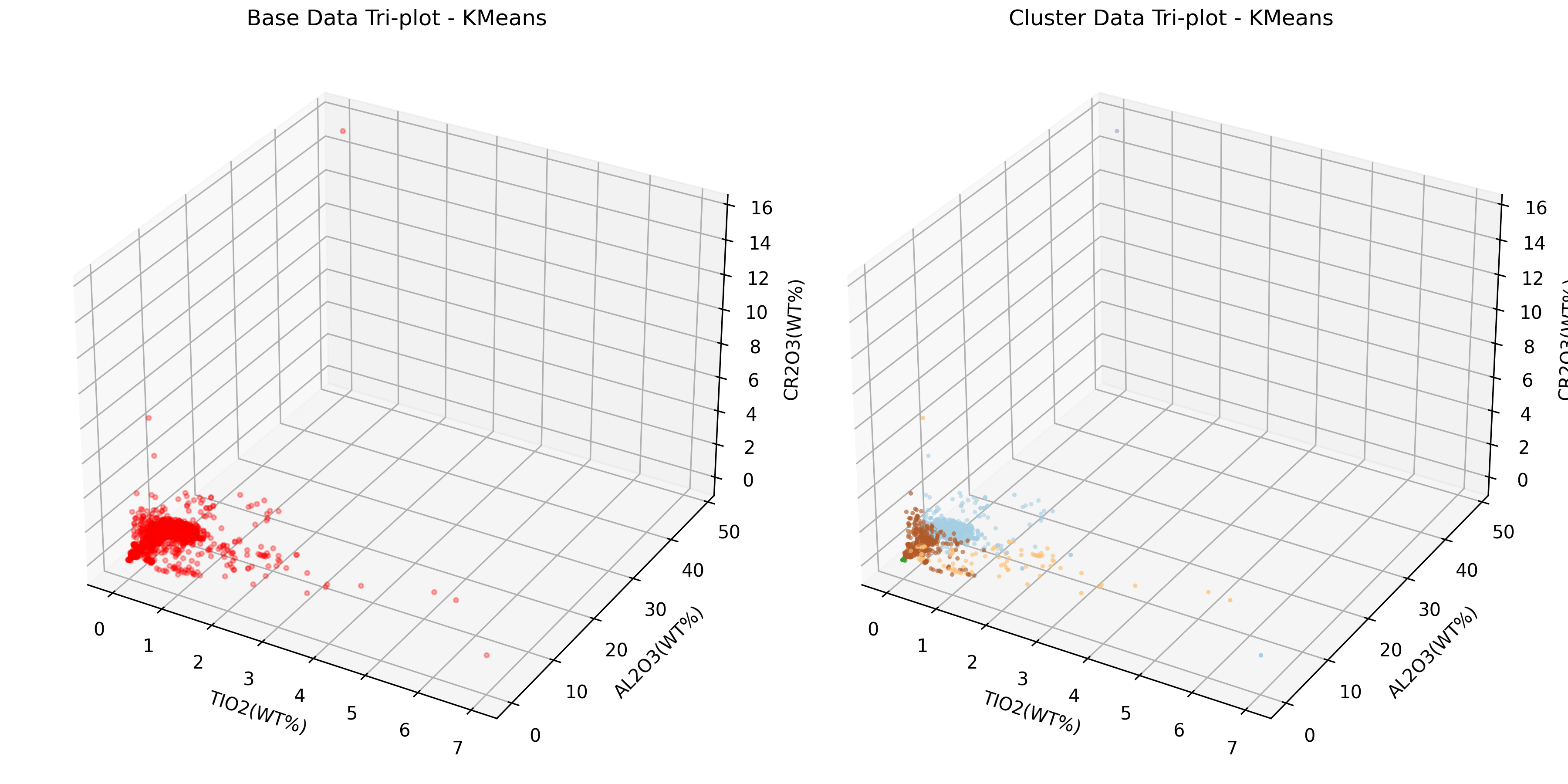
-----* Cluster Three-Dimensional Diagram *-----
Save figure 'Cluster Three-Dimensional Diagram - KMeans' in
C:\Users\YSQ\geopi_output\n\test2\artifacts\image\model_output.
Successfully store 'Cluster Two-Dimensional Diagram - KMeans' in 'Cluster Two-Dimensional Diagram - KMeans.xlsx' in
C:\Users\YSQ\geopi_output\n\test2\artifacts\image\model_output.
-----* Clustering Centers *-----
[[5.41388401e+01 2.15829364e-01 1.29914717e+00 4.67482921e-01
3.19637435e+00 2.35938062e+01]
[5.22315058e+01 3.33761788e-01 4.56573367e+00 8.00137780e-01
3.03767947e+00 2.14858778e+01]
[4.47251667e+01 5.05000000e-02 1.58216667e+00 9.81666667e-02
9.22933333e+00 4.75750000e-01]
[5.08836094e+01 6.82282120e-01 6.77641282e+00 8.42755279e-01
3.40927321e+00 2.05098654e+01]
[2.18000000e-01 1.63000000e-01 4.82230000e+01 1.54210000e+01
1.54690000e+01 1.09000000e-01]]
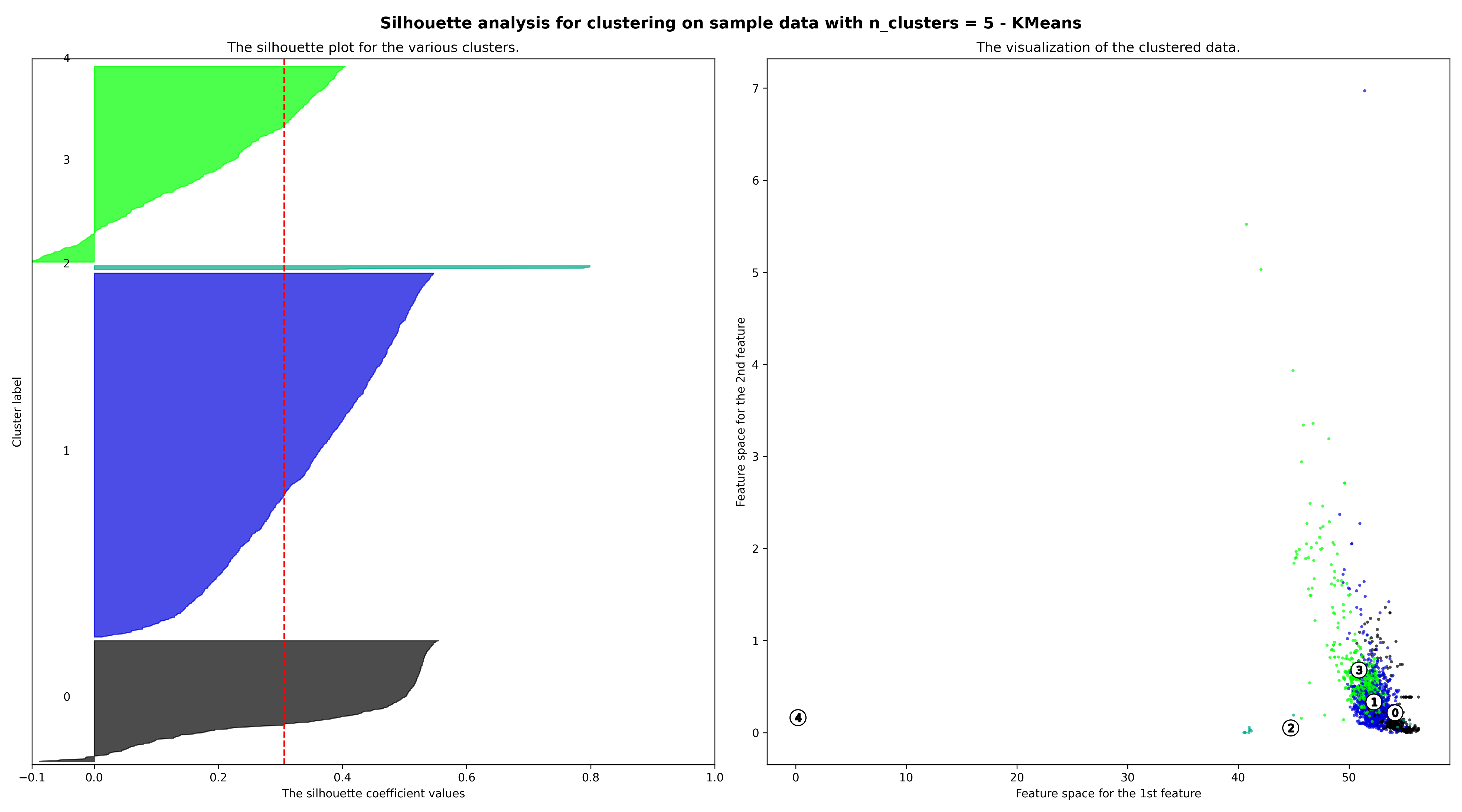
-----* Silhouette Diagram *-----
For n_clusters = 5 The average silhouette_score is : 0.30630378777495465
Save figure 'Silhouette Diagram - KMeans' in C:\Users\YSQ\geopi_output\n\test2\artifacts\image\model_output.
Successfully store 'Silhouette Diagram - Data With Labels' in 'Silhouette Diagram - Data With Labels.xlsx' in
C:\Users\YSQ\geopi_output\n\test2\artifacts\image\model_output.
Successfully store 'Silhouette Diagram - Cluster Centers' in 'Silhouette Diagram - Cluster Centers.xlsx' in
C:\Users\YSQ\geopi_output\n\test2\artifacts\image\model_output.
-----* Silhouette value Diagram *-----
Save figure 'Silhouette value Diagram - KMeans' in C:\Users\YSQ\geopi_output\n\test2\artifacts\image\model_output.
Successfully store 'Silhouette value Diagram - Data With Labels' in 'Silhouette value Diagram - Data With Labels.xlsx'
in C:\Users\YSQ\geopi_output\n\test2\artifacts\image\model_output.
-----* KMeans Inertia Scores *-----
Inertia Score: 12567.410753356708
Successfully store 'KMeans Inertia Scores - KMeans' in 'KMeans Inertia Scores - KMeans.txt' in
C:\Users\YSQ\geopi_output\n\test2\metrics.
-----* Model Persistence *-----
Successfully store 'KMeans' in 'KMeans.pkl' in C:\Users\YSQ\geopi_output\n\test2\artifacts\model.
Successfully store 'KMeans' in 'KMeans.joblib' in C:\Users\YSQ\geopi_output\n\test2\artifacts\model.
(Press Enter key to move forward.)
```
```
-*-*- Transform Pipeline Construction -*-*-
Build the transform pipeline according to the previous operations.
Successfully store 'Transform Pipeline Configuration' in 'Transform Pipeline Configuration.txt' in
C:\Users\YSQ\geopi_output\n\test2\artifacts.
(Press Enter key to move forward.)
> Enter
```
<font color=gray size=1><center>Figure 1 Silhouette Diagram - KMeans</center></font>
<font color=gray size=1><center>Figure 2 Cluster Two-Dimensional Diagram - KMeans</center></font>
<font color=gray size=1><center>Figure 3 Cluster Three-Dimensional Diagram - KMeans</center></font>
The final trained Kmeans models will be saved in the output/trained_models directory.